Every gradient step during training is an estimate. We can’t compute the true gradient since it’s too costly to compute for each sample in the dataset. Thus, we approximate it from a mini-batch. The approximation introduces noise, and the amount depends on the batch size. Too small, our estimate is noisy; too large, and you waste compute for reduced gains.

Let’s consider G to be our true gradient computed from the average of gradients from every sample. Since this G is hard to compute, we take random samples and estimate ĝ,

Under a locally quadratic model of the loss, the expected behavior of a step depends only on the first two moments of the gradient estimate: its mean and spread (variance). So we can describe batch behavior entirely in terms of those two.

1^st Moment: Mean

Since each sample in the mini-batch is drawn i.i.d. from the dataset, we can decompose the expectation directly:

ĝ​ is an unbiased estimator of G. The unbiasedness tells us our estimates are centered on the true gradient, but we wouldn’t know the deviation of our draws from truth; we can denote the deviation “noise” (or shortened: “ε”).

As B → ∞, this deviation vanishes — the estimate recovers the true gradient exactly.

To characterize this noise we follow the bilinearity of the covariance to decompose the per-sample covariance giving us the covariance of our gradient estimate.

2^nd Moment: The Spread

Given our earlier definition of error, our gradient estimate can be easily decomposed into mean (true gradient) and noise (deviation from true gradient). Under the assumption that we did i.i.d sampling our error term would be roughly centered around the same mean (true gradient). Our gradient estimate covariance is proportional to error covariance.

Where Cov(g) is the per-sample gradient covariance matrix. Since our true gradient in our interpretation is the mean gradient that we would get if we trained with bs of inf, only our noise term will account for the explained variance, thus, our noise covariance ends up reducing to E[εε^T] scaled by 1/B.

Now we have both moments. The noise covariance scales as 1/B, doubling the batch halves the noise covariance i.e the estimate is closer to true gradient (tighter around the true gradient).

Plugging this to our update rule we get:

The Squared Norm

Our update now is a vector with two components, signal and noise. We still have to estimate how much of a step is useful, which requires us to choose a norm and its corresponding metric.

SGD implicitly treats parameter space as flat Euclidean space, the update is the gradient, with no reweighting of directions. That choice of geometry gives us the natural energy measure: the Frobenius/L2 norm. (An optimizer like Adam uses per-coordinate metric, which is why we can’t directly apply this derivation for adam/rms-prop family optimizers).

Check out Old Optimizer, New Norm: An Anthology for derivation of norms for some of the popular optimizers.

Plugging our decomposition ĝ​ = G + ε̂ into the expected squared norm of the gradient estimate:

Since E[ε̂] = 0 (because of our unbiased estimator for G), we discard the cross correlation term. Our expected squared norm of ε̂ transforms into the total variance of g.

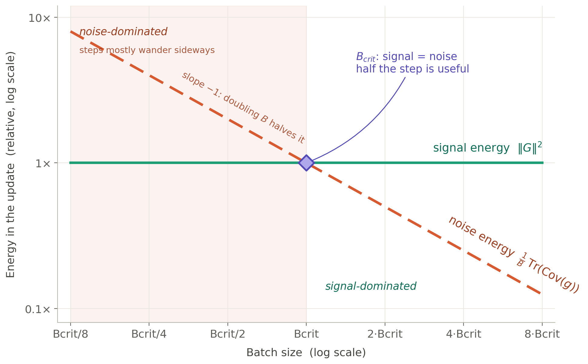
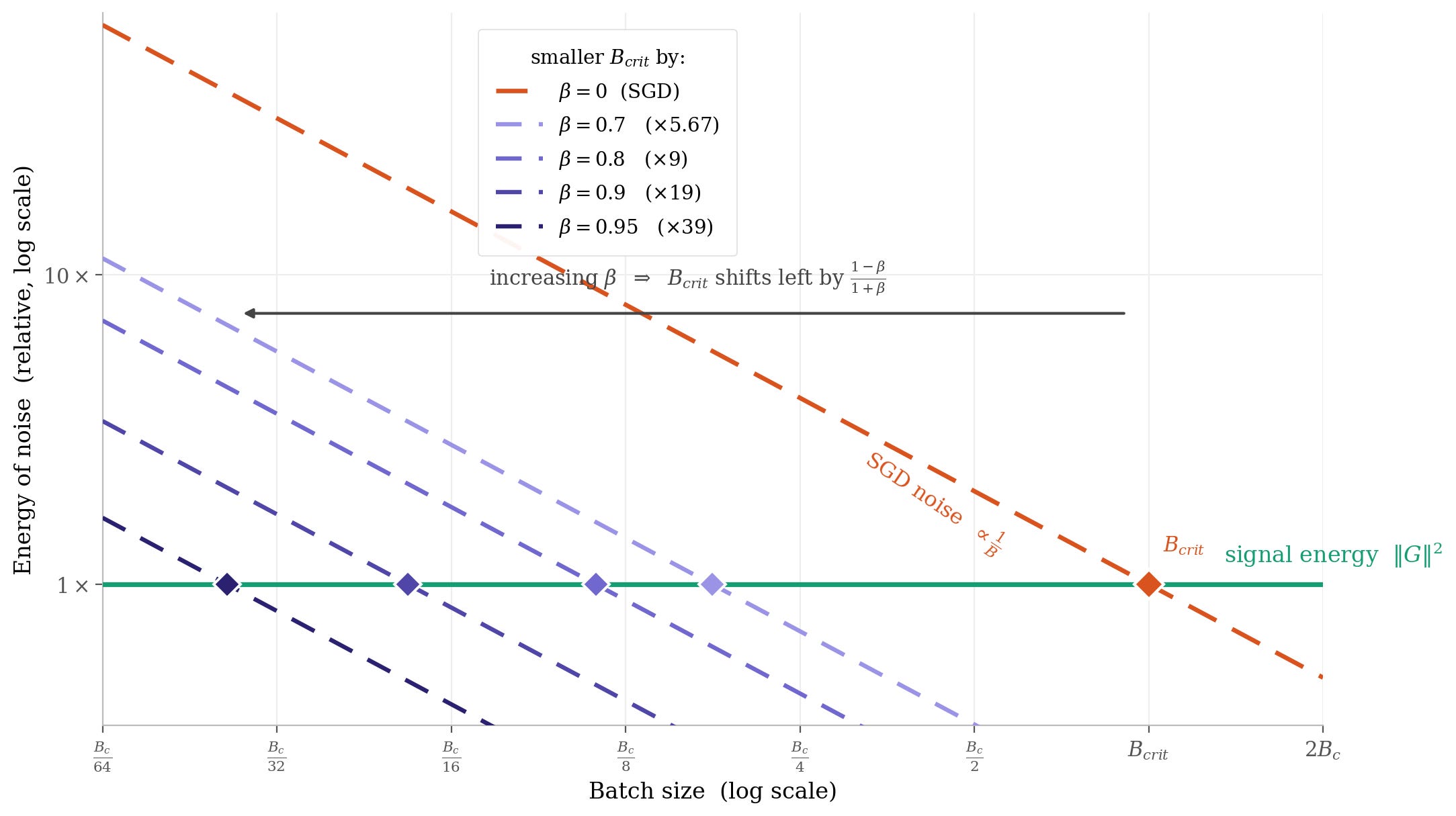
Further we can define critical batch size at which point signal energy is equal to noise energy.

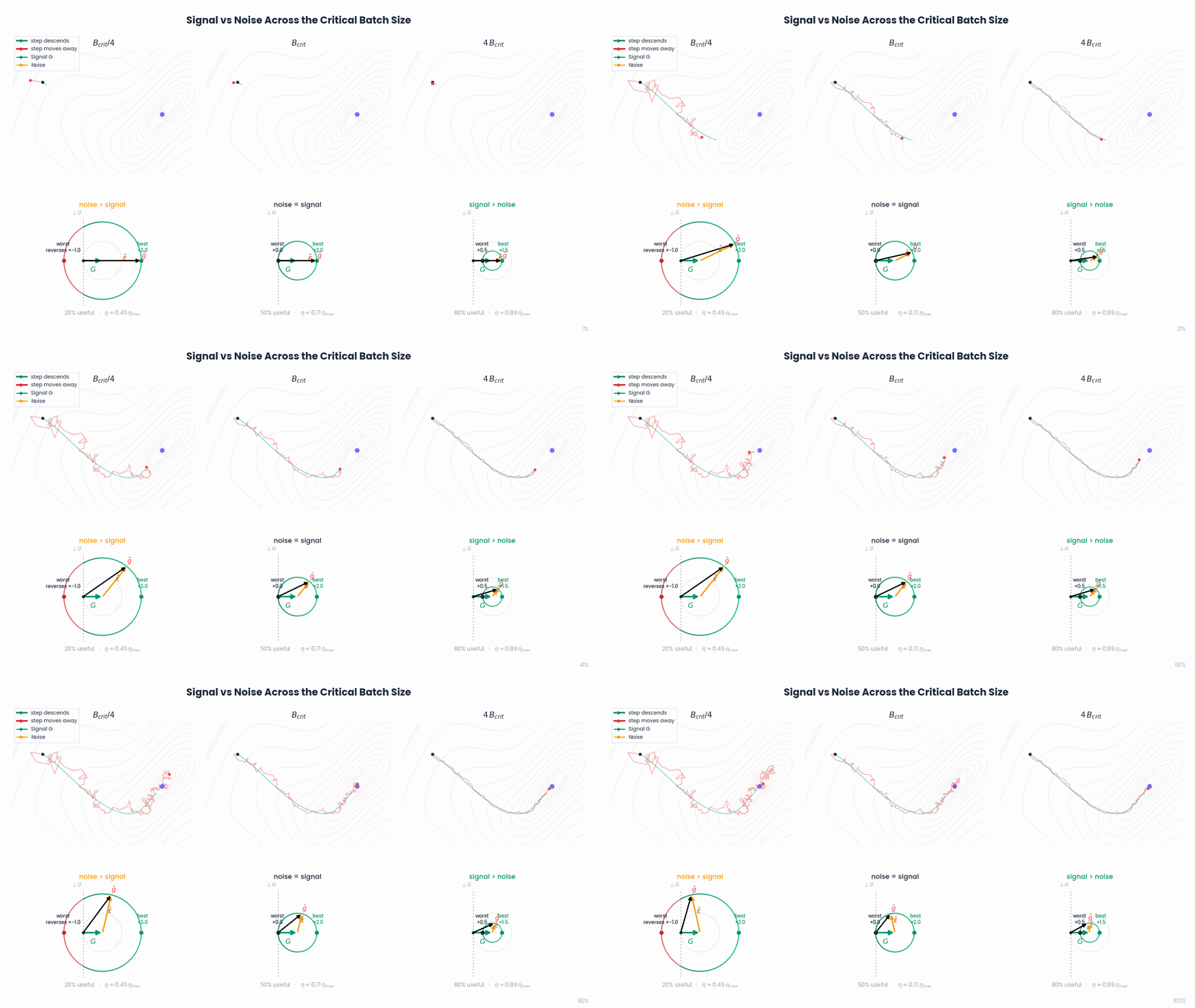
Looking at this ratio, B_crit defines the point at which signal is no longer dominated by noise, since ||G||² is our true gradient’s energy its invariant to our batch size and is constant, but ||ε||² is a function of our batchsize and scales by 1/B as we derived earlier. Further details on economical batchsize below.

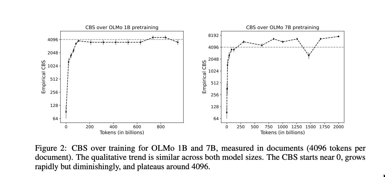
At this point it’s intuitive that the critical batch size is not stationary, its a function of gradient at every point, Since early in the training we per-sample gradients often point to the same direction, ||G||² >> Tr(Cov(g)) (True gradient energy is larger than gradient noise) our critical batch size starts at ~0. As we carve out the loss landscape we get a more anisotropic landscape, the noise energy starts climbing as only few components of our estimated gradient agree with the true gradient, this increases our critical batch size.

This paper namely has explicitly noted the approach they used to calculate the cbs might not be optimal under adam family optimizers thus these observations might be conflated.

Incorporating the Learning Rate

In most deep learning methods, we are not regressing on linear functions — and the Gradient Descent assumption is that even if the loss geometry is highly non-linear, if you discretize it enough it becomes somewhat flat, the discretization window kernel is our step-size/lr/“η”.

Further even with provided step budget / trust region “η”, that was only under a noise-less regime, as B → ∞. Below that regime we would in worst case be stepping on the noise’s direction rather than our true gradient’s. Thus usable lr should be derived from our critical batchsize estimate.

After these adjustments, our update becomes Δθ=−ηĝ instead of Δθ=−ĝ

Further we can denote S² = E∥Δθ∥². S is the RMS step length you've budgeted per update, our trust-region radius. And then we estimate the learning rate coupling with batch size:

Define η_max⁡ = S/∥G∥ as the ratio of step budget and true gradient norm, this under low noise (i.e. B→∞) regime saturates at “η” and trends towards 0 at high noise (i.e. B→1).

Then the relationship simplifies to:

Our lr scaling rule fixes a single step-size budget on ‖Δθ‖ — a uniform trust region in primal space, and solving that length constraint puts the noise under a square root, giving √B scaling. McCandlish et al. instead maximize the expected per-step loss decrease, an objective whose optimum puts the noise in the denominator directly, so it scales linearly in B;

$$\eta_{opt}(\mathbf{\textcolor{blue}{B}}) = \frac{\eta_{max}}{(1+\frac{B_{crit}}{\mathbf{\textcolor{blue}{B}}})}$$

This gives us clean regime separation:

• B << B_critical — Noise-dominated.

  • Here B_critical/B >> 1, thus the signal term (1) has proportionally less impact on the sqrt term. As B climbs from ≪B_crit to B_crit, the signal's share of the update energy rises from near 0 to 50%.

    $$\eta(\mathbf{\textcolor{blue}{B}}) = \frac{\textcolor{green}{\eta_{max}}}{\sqrt{1 + \frac{B_{crit}}{\mathbf{\textcolor{blue}{B}}}}} \qquad \underset{\frac{B_{crit}}{\mathbf{\textcolor{blue}{B}}} \gg 1}{\approx} \qquad \textcolor{green}{\eta_{max}}\cdot\sqrt{\frac{\mathbf{\textcolor{blue}{B}}}{B_{crit}}} = \frac{\textcolor{green}{\eta_{max}}}{\sqrt{B_{crit}}}\cdot\sqrt{\mathbf{\textcolor{blue}{B}}}$$

  • The usable learning rate is small and grows like √B — every doubling of the batch increases by a full factor of √2 in usable LR. Compute spent on a larger batch pays off at the best rate it ever will.

• B = B_critical​ — The crossover.

  • Your usable LR is η(B_crit) = η_max/√2 = S/(√2·‖G‖) ≈ 0.71·η_max — the step budget over √2 times the gradient norm.

• B >> B_critical — Signal-dominated.

  • Now B_crit/B → 0, so η(B) → η_max and the usable learning rate saturates.

    $$\eta(\mathbf{\textcolor{blue}{B}}) = \frac{\textcolor{green}{\eta_{max}}}{\sqrt{1 + \frac{B_{crit}}{\mathbf{\textcolor{blue}{B}}}}} \qquad \underset{\frac{B_{crit}}{\mathbf{\textcolor{blue}{B}}} \ll 1}{\approx} \qquad \textcolor{green}{\eta_{max}}\left(1 - \frac{B_{crit}}{2\mathbf{\textcolor{blue}{B}}}\right) \xrightarrow[\;\mathbf{\textcolor{blue}{B}} \to \infty\;]{} \textcolor{green}{\eta_{max}}$$

  • Each doubling of the batch increases the usable LR by a factor strictly less than √2, trending toward 1. We’re paying linearly more compute for sub-linearly more per-step progress, i.e diminishing returns (more on the economical side of this below).

Why noise dominance hurts?

The regime boundary isn’t a superfluous concern, optimization steps under that regime actively degrades our optimization process.

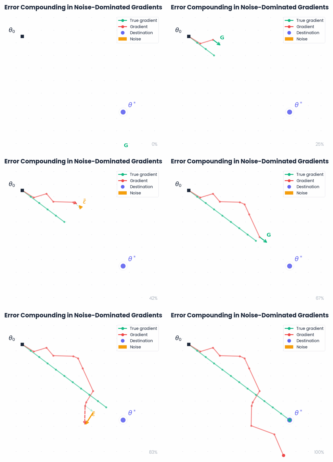
When B << B_critical, our gradient estimate ĝ is mostly ε̂. The update pushes θ toward the region carved by ε̂ rather than toward θ - ηG. But it doesn't stop there: once you've landed at θ′ shaped by ε̂, the next gradient you compute at θ′ has its own ε̂, and that new ε̂ pushes you further from the trajectory you'd have taken under the true gradient. The errors compound.

In high dimensions, the noise component often has little projection onto the true gradient direction. So when noise energy dominates, much of the update budget is spent moving sideways rather than descending.

Momentum

One option to get a better estimate of G is to keep an exponential moving average of our gradients, i.e Momentum SGD.

Unrolling the recursion, momentum is a geometrically weighted sum of our past gradient estimates.

Computing the B_critical for this:

We can further plug this estimate into optimal lr calculation, but for brevity I’ll conclude the derivations here.

G is approximately constant over the EMA window scale β. True only when the loss landscape isn't changing faster than the momentum timescale ~1/(1−β).

Noise is white in time: E[ε̂_{t−i}ε̂_{t−j}ᵀ]=0 for i≠j, each with covariance Σ/B. Real consecutive minibatches have correlated gradients, so this is the optimistic casel. But this is not always the case, thus the true SNR gain is lower.

Economical-CBS

Of course we can just use gradient accumulation to hit any batch size we want, right? Accumulate micro-batches, sum the gradients, step once. Mathematically equivalent to a larger batch.

The problem is that hardware doesn’t have instant transfer and instant bandwidth between SMs, HBM, caches, threads and registers. No matter how accurate to math we have to adhere with physical limitation and so we need a new point of view, I’ll haphazardly call this Economical-CBS.

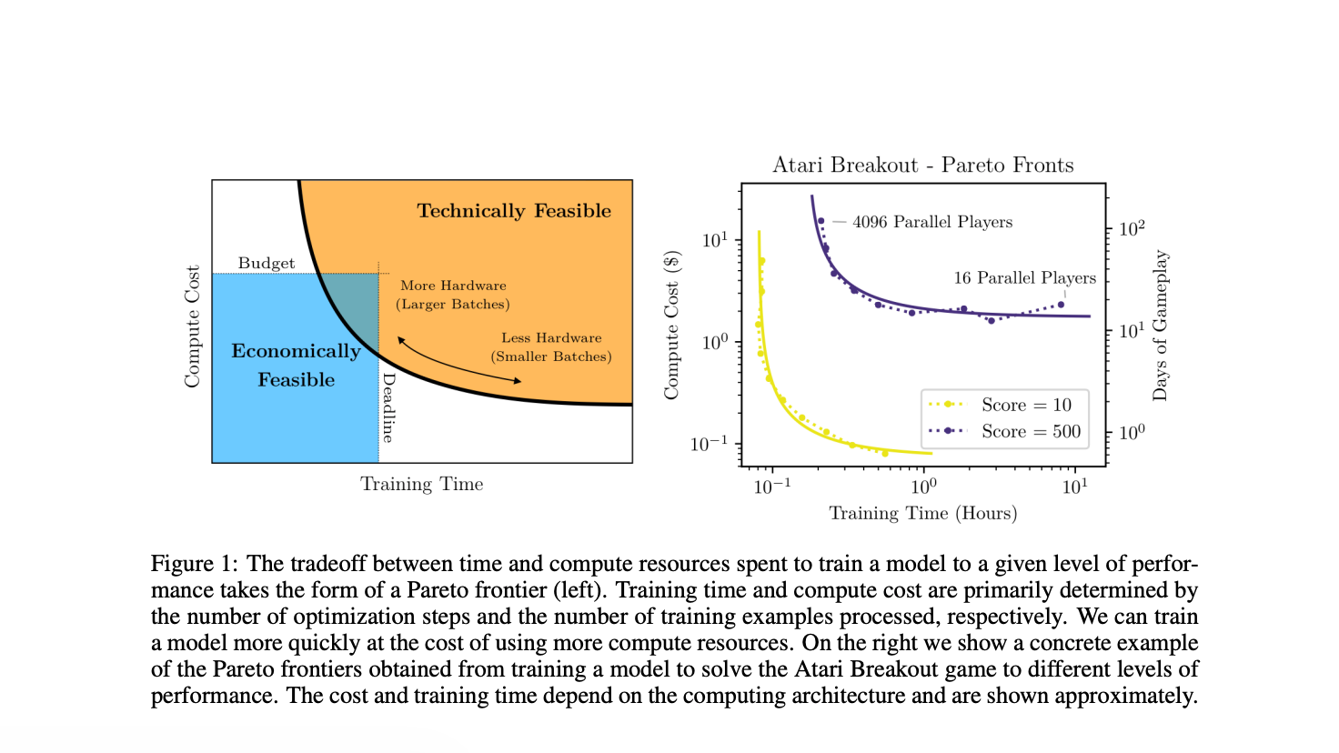
I won't derive the full economical CBS here, for that, check out An Empirical Model of Large-Batch Training by McCandlish et al., from which the famous batch size scaling graph comes.

The economical CBS maximizes training progress per unit of wall-clock time (or per dollar) instead of gradient step. It accounts for the throughput curve of your specific hardware. Below the economical CBS, you’re leaving compute on the table. Above it, you’re paying linearly more time for sub-linearly more progress.

Conclusion

Good optimization lives in a small quadrant of several hyperparameters, often times unforgiving. B_crit itself depends on where you are in training, which means the optimal batch size shifts, which is part of why hyperparameter tuning is so fragile.

To remedy this people often rely on existing architectures and recipes to avoid paying for cost of exploration. But this reduces the novel behaviors we could exploit.

Several works try to remedy this with hyperparameter transfer methods such as μP, depth-μP and lr-free optimizers such as D-adapt (which estimate the lr using running eta estimates), but we are yet to see a truly general method that’s competitive to hand-tuned baselines.

PS: This post was originally a part of another blog on optimizer ontology, but decided to separate it for being orthogonal to the basis I chose, but more to come…

PS: Substack is really inconvenient for writing math notations and latex, I’m yet to determine whether or not its a skill issue on my side.

Thanks to Adina Pak, Francesco, Stefan, Cyris, Lucas for reading early draft of this post, furthermore thanks to my friends Simo Ryu, Kevin Yin for inspiring this topic many moons ago.